Parametric Design Optimization for Carbon Fiber Composite Parts: FEA Software and Workflow Guide Parametric design optimization has become an indispensable methodology in carbon fiber composite engine...
Parametric Design Optimization for Carbon Fiber Composite Parts: FEA Software and Workflow Guide
Parametric design optimization has become an indispensable methodology in carbon fiber composite engineering, enabling structural engineers to systematically explore design alternatives that simultaneously satisfy mass targets, strength requirements, manufacturing constraints, and cost limitations. Unlike traditional iterative design approaches that rely heavily on engineering judgment and manual reanalysis, parametric optimization uses mathematical programming algorithms to automatically search the design space for optimal solutions, dramatically reducing development time and improving final part quality.
For carbon fiber composite parts, the optimization challenge is uniquely complex due to the additional design variables introduced by laminate architecture — ply orientations, stacking sequences, ply drop-offs, and material selection — beyond the geometric parameters typical of metallic component design. A typical automotive CFRP component optimization involves 50–200 design variables, compared to 10–30 for an equivalent steel component.
Optimization Framework Overview
A complete parametric design optimization workflow for CFRP parts consists of four interconnected stages:
- Parameterization — Defining the design variables that describe the part geometry, laminate layup, and manufacturing process
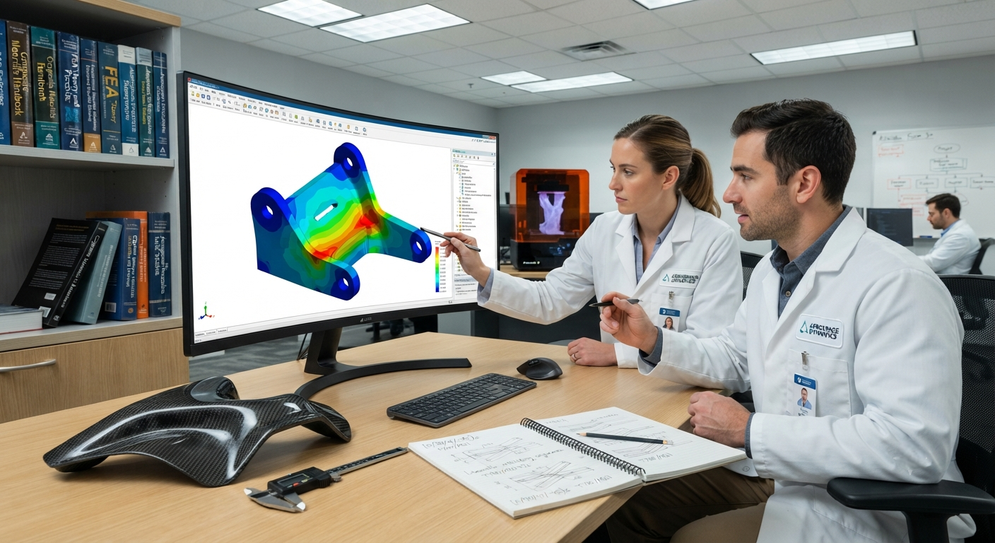
- Simulation — Finite element analysis (FEA) of structural performance under specified loading conditions
- Optimization — Mathematical programming that iteratively adjusts design variables to minimize or maximize an objective function while satisfying constraints
- Post-processing — Validation, manufacturability assessment, and final design release
Leading FEA Software Solutions for CFRP Optimization
| Software | Developer | Optimization Type | Composite-Specific Features | License Cost (annual) |
|---|---|---|---|---|
| OptiStruct | Altair | Topology, topography, size, shape, free-size, free-shape | Ply-based optimization, failure criteria (Tsai-Wu, Puck, Hashin), manufacturing constraints (draw direction, symmetry, core) | $18,000–$45,000 |
| ANSYS Composite PrepPost (ACP) + DesignXplorer | Ansys | Response surface, direct, multi-objective genetic algorithm | Layered composite modeling, sandwich design, failure analysis, progressive damage | $12,000–$38,000 |
| Abaqus FEA + Tosca | Dassault Systèmes | Topology, shape, sizing, bead optimization | Anisotropic material support, cohesive zone modeling, mesh-independent optimization | $25,000–$60,000 |
| Digimat | e-Xstream (Hexagon) | Multi-scale material optimization, injection molding-linked | Micro-mechanics, fiber orientation prediction, warpage compensation | $15,000–$40,000 |
| HyperSizer | Collier Research | Size optimization, laminate blending, panel buckling | NASA-developed composite sizing, extensive material database, automated laminate reporting | $20,000–$35,000 |
| FiberSIM | Synera (formerly Siemens) | Manufacturing-focused optimization for AFP and ATL | Drape simulation, tow steering, cut-path optimization, scrap minimization | $8,000–$25,000 |
Workflow: Step-by-Step Guide
Stage 1: Problem Definition and Parameterization
The foundation of any parametric optimization is the correct definition of design variables. For a CFRP component, these must be carefully categorized:
- Geometric variables — thickness distributions, rib heights, draft angles, fillet radii, hole locations. Typical range: 10–40 variables
- Laminate variables — ply orientation angles (integer 0°, ±45°, 90°), ply count per orientation, stacking sequence, core thickness. Typical range: 20–100 variables
- Material variables — fiber type selection (T300, T700, IM7, M40J), matrix type (epoxy, PEEK, BMI), fabric architecture (UD tape, woven, NCF). Typical range: 5–15 variables
- Manufacturing variables — mold temperature profile, injection pressure, vacuum level, cure cycle duration. Typical range: 5–20 variables
Design variable screening using design of experiments (DoE) methods — fractional factorial or Plackett-Burman designs — should be performed first to identify the most influential variables and reduce the dimensionality of the optimization problem. A typical screening exercise can reduce the variable count by 40–60% without significant loss of design fidelity.
Stage 2: FEA Model Setup
For composite FEA, element selection and material property definition are critical. Shell elements with composite layup definitions (e.g., Abaqus S4R or ANSYS SHELL181 with sections) are standard for thin-walled CFRP parts. Solid elements (Abaqus C3D8R or ANSYS SOLID185) are required for thick laminates (>10 mm) or where through-thickness stresses matter, such as bolted joint regions.
Material properties must be specified as orthotropic elastic constants (E₁, E₂, G₁₂, ν₁₂) with corresponding strength values (Xₜ, X꜀, Yₜ, Y꜀, S) for each candidate material system. Failure criteria selection — Tsai-Wu (quadratic interactive), Hashin (mode-separating), or Puck (physically based) — significantly impacts optimization results and should be selected based on the dominant failure modes expected in the application.
Stage 3: Optimization Execution
Multi-objective optimization is standard for CFRP parts, balancing competing objectives such as:
- Minimize mass (primary objective in most automotive and aerospace applications)
- Maximize stiffness (maintaining deflection within allowable limits)
- Minimize cost (factoring raw material, tooling, and cycle time costs)
- Maximize manufacturability (ensuring compliance with AFP/ATL or HP-RTM process constraints)
- Maximize damage tolerance (using residual strength after impact as a constraint)
For multi-objective problems, the Non-dominated Sorting Genetic Algorithm II (NSGA-II) has become the industry-standard optimizer for composite laminate problems, consistently outperforming gradient-based methods for discrete ply-angle optimization. Response surface methods (Kriging, Radial Basis Functions) are effective for problems with 20–50 continuous variables but degrade above 100 variables without dimensionality reduction.
Stage 4: Results Interpretation and Validation
After optimization convergence — typically requiring 500–5,000 FEA evaluations depending on variable count and problem complexity — the Pareto frontier of optimal designs must be reviewed. Key validation steps include:
- Checking ply continuity and manufacturability (no dropped plies that violate stacking sequence rules)
- Verifying that optimized ply angles conform to standard orientation sets (0°, ±45°, 90°)
- Confirming inter-laminar shear stresses remain within allowable limits
- Validating against a high-fidelity FEA model with refined mesh at critical regions
- Physical testing of representative prototype specimens for correlation
Frequently Asked Questions
What is the typical time savings from using parametric optimization versus traditional iterative design for CFRP parts?
For a moderately complex CFRP component — such as an automotive suspension control arm or aerospace bracket — parametric optimization typically reduces engineering development time by 40–65%. A traditional iterative approach requiring 8–12 design loops over 6–8 weeks can be completed in 2–3 weeks using parametric optimization with a properly parameterized FEA model. The savings are largest for parts requiring composite-specific optimization (ply orientation and stacking sequence) where the design space is too large for manual exploration.
Can parametric optimization handle manufacturing constraints like AFP tow steering limitations?
Yes. Modern optimization software integrates manufacturing constraints through penalty functions or constraint definitions. For automated fiber placement (AFP), constraints include minimum tow length (typically 50–100 mm), maximum steering radius (500–3,000 mm depending on tow width), allowable gap and overlap between adjacent tows (±0.5 mm), and ply drop-off rate (maximum 1 ply per 10 mm step). Altair OptiStruct and Synera FiberSIM both support AFP-aware optimization that automatically generates ply boundaries respecting these constraints, reducing the gap between the optimized design and the as-manufactured part.
What is the recommended approach for optimizing hybrid (CFRP + metal) joints within a parametric framework?
Hybrid joint optimization requires a multi-scale approach. At the macro level, the optimization defines the joint location, overlap length (typically 30–50 mm for bonded joints), fastener spacing (4–6× fastener diameter), and laminate thickness buildup around the joint. At the micro level, the optimization selects the adhesive type (epoxy vs. polyurethane), surface treatment method (peel ply vs. plasma vs. laser ablation), and fastener material (aluminum vs. titanium vs. stainless steel). The recommended workflow uses a submodeling technique — a coarse global model drives overall geometry and laminates, while a refined local submodel optimizes the joint details with cohesive zone elements (CZM) for accurate strength prediction.
What FEA solver is best for large-scale composite optimization (200+ design variables)?
For large-scale composite optimization problems with 200+ design variables, Abaqus FEA coupled with Tosca (for topology optimization) or OptiStruct (for laminate sizing) are the most capable commercial solvers. Both support distributed parallel computing across multiple CPUs and GPU-accelerated solvers for linear static and eigenfrequency analysis. Ansys Mechanical APDL with DesignXplorer is also effective when using response surface optimization (RSM) with design of experiments (DoE) to reduce the effective optimization dimension. For problems exceeding 500 variables, two-level optimization approaches — where topology optimization identifies the load-path geometry first, followed by detailed laminate sizing — are strongly recommended to maintain practical computation times (typically under 72 hours on a 32-core workstation).
Part of topic
Related Articles
- Bio-Based Carbon Fiber Precursors: Lignin and Polyethylene for Low-Cost Production
- Large-Tow Carbon Fiber Cost Analysis: 48K vs 60K Price-Performance Comparison
- Carbon Fiber-Resin Interface Bonding: Surface Treatment and Coupling Agent Optimization
- Digital Twin for Carbon Fiber Manufacturing: Real-Time Process Monitoring and Defect Prevention
- Thermoplastic Carbon Fiber Welding for Automotive: Ultrasonic and Induction Welding Process Windows
- Large-Tow Carbon Fiber Wet Spinning: Process Optimization for 48K/60K Production Efficiency
Interested in Our Products?
Contact our team for competitive pricing and technical specifications.
Get a QuoteRelated Products
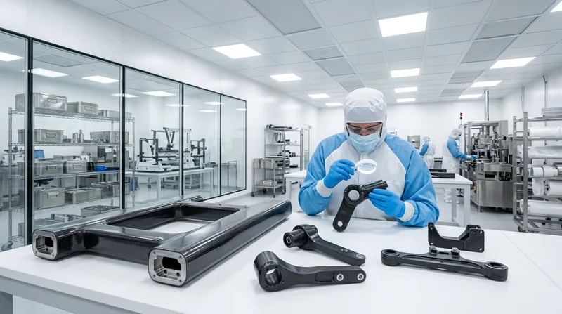
Custom Carbon Fiber Medical Device Components
Medical-grade carbon fiber components manufactured for imaging equipment, surgical instruments, and patient support systems. Carbon fiber's radiolucency (X-ray transparency) and high strength-to-weight ratio make it ideal for CT scanner beds, wheelchair frames, surgical robot arms, and MRI-compatible accessories. Biocompatible resin systems available.
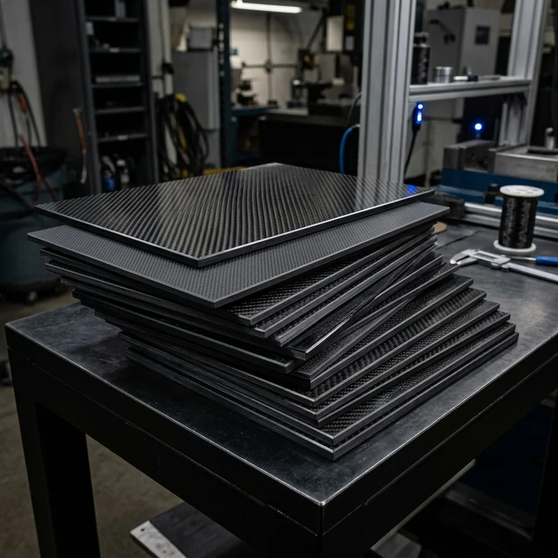
Carbon fiber standard plate-3k stripe
Lightweight, ultra-rigid standard sheets for drone fuselages, robot housings, facades and structural applications.
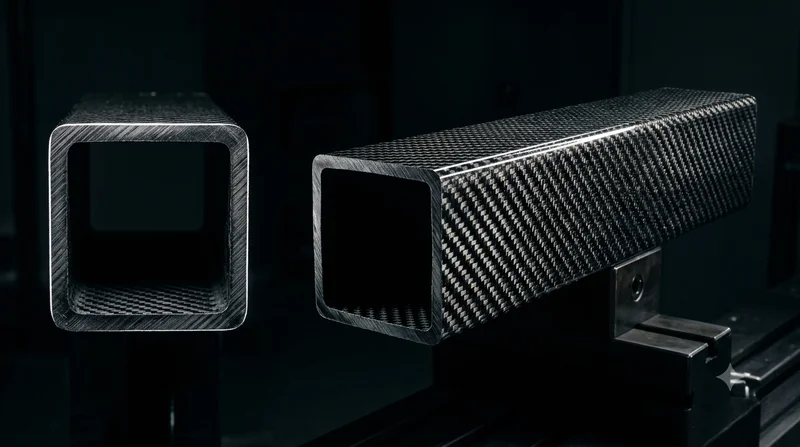
Square Carbon Fiber Tube — 3K Twill T700
Square cross-section carbon fiber tube manufactured with 3K twill weave for torsional strength. Preferred for structural frames, trusses, and support columns where rectangular geometry offers design flexibility.
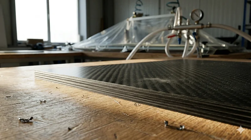
Carbon Fiber Plate — 3K Twill T700 3.0mm
Medium-thickness 3.0mm carbon fiber plate offering significantly higher load capacity while maintaining attractive 3K twill finish. Suitable for structural brackets, reinforcement plates, and load-bearing panels.
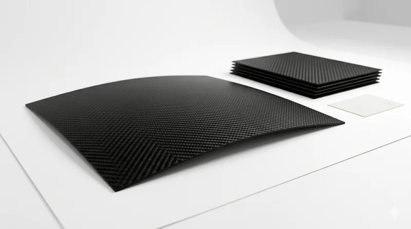
Carbon Fiber Plate — 3K Twill T700 1.5mm
Thin 1.5mm carbon fiber plate with 3K twill weave surface. Lightweight and stiff, commonly used for covers, panels, drone bodies, and applications requiring a premium aesthetic appearance.